Home Announcements Discussion Board (DB) Objectives Pacing Guides FAQs Grades Calculators

Course Announcements

Week 1 Week 2 Week 3 Week 4 Week 5

Week 6 Week 7 Week 8 Week 9 Week 10

Week 11 Week 12 Week 13 Week 14 Week 15

Welcome to Week 1: Limit and Continuity of Functions

Great Students,

Greetings to everyone.
Welcome to Module 1.

Have you heard of these terms:
elastic limit (Physics: Hooke's Law anyone)?
weight limit (Kinesiology: Where are the fitness/muscular guys?)
speed limit (Raise your hand if you've never gotten a speeding ticket)
Literally speaking, limit refers to a bound.
What happens if the limit is exceeded?

Recall in: Algebra:
$y = f(x)$
x = input or independent variable
y = output or dependent variable or function value

Evaluating Functions (Function Values): What is the value of the output if the input is a specific value?
For example: say that:

$ f(x) = x^2 - 3 \\[3ex] \text{Find } f(4) \\[3ex] f(4) = 4^2 - 3 \\[3ex] f(4) = 16 - 3 \\[3ex] f(4) = 13 \\[3ex] $ Now onto: Calculus:
Limits: What does the value of the output approach to, as the input approaches a specific value?
Following the same example,
If $x = 3.9, 3.99, 3.999, 3.9999, ...$, what are the values of $f(x)$?
In other words, as x approaches 4 from the left, what does $f(x)$ approach to?
That value is known as the Left-Hand Limit of the function.

Similarly, If $x = 4.1, 4.01, 4.001, 4.0001, ...$, what are the values of $f(x)$?
In other words, as x approaches 4 from the right, what does $f(x)$ approach to?
That value is known as the Right-Hand Limit of the function.

Do you get the idea?
Do you want some real-world examples?


Academic Scenario:
(1.) Let's assume that for the male student, Student A:
(a.) He is required to take a test every week on Friday.
(b.) To prepare for the test on Friday, He needs to study from Monday through Thursday.
Let's assume again that the average person can study effectively for about 3 to 5 hours daily.
This implies a weekly study range of about 12 to 20 hours before taking the test.
In this scenario, 20 hours is the limit.

Student A wants to determine if there is any relationship between his study hours and his test grade.
Does the number of study hours have any effect on his grade?
The study hours is the independent variable (input).
The test grade is the dependent variable (output).

If Student A:
studies for 12 hours, what is his test grade?
studies for 13 hours, what is his test grade?
studies for 14 hours,..., what is his test grade?
Mathematically speaking, we can say any of these:
What is the test grade of Person A as his study hours approaches (but does not reach) 20 hours?
What is the left-hand limit of Person A's test grade as his study hours approaches (but does not equal) 20 hours?
Let's say that the grades keep improving as his study hours increase.
This implies a continuous improvement in his grades.
But, what if Student A skips studying on Monday, Tuesday, and Wednesday; and rushes and crams a lot of notes on Thursday for 19 hours?
What do you think about his grade? (Did you think about discontinuity?)

Business Scenario:
Person B sells shirts.
When the shirt is marked at $5, about 50 shirts are sold each week.
So, the function value = 50 shirts.
She wants to explore if there is a relationship between the price of a shirt and the number of shirts she sells.
How many shirts are sold if the shirt is marked at:
$3.00
$3.50
$4.00
$4.50
In other words, what is the left-hand limit (LHL) of the number of shirts sold as the price approaches $5?

Also, how many shirts are sold if the shirt is marked at:
$7.00
$6.50
$6.00
$5.50
In other words, what is the right-hand limit (RHL) of the number of shirts sold as the price approaches $5?

If the Left-Hand Limit = Right-Hand Limit = Function Value = 50 shirts, then the function is continuous at $5.
But, what if Person B runs a special promotion of BOGO (Buy one, Get one) free at the price of $5, how will it affect the sales?

Welcome to Limit and Continuity of Functions.

May you please:
(1.) Click the Week 1 module.
(2.) Review the Learning Objectives.
(3.) Review the Readings/Assessments.
(4.) Complete the assessments initially due this week.
(5.) Participate in the Week 1 Discussion (DB 1).
(6.) Attend the Live Sessions/Student Engagement Hours for this week.

Should you have any questions, please ask. I am here to help.
Thank you.

Samuel Chukwuemeka
Working together for success


Welcome to Week 2: Average Rate of Change

Great Students,

Greetings to everyone.
Welcome to Module 2.

In Module 1, we discussed the topics of Limits and Continuity.
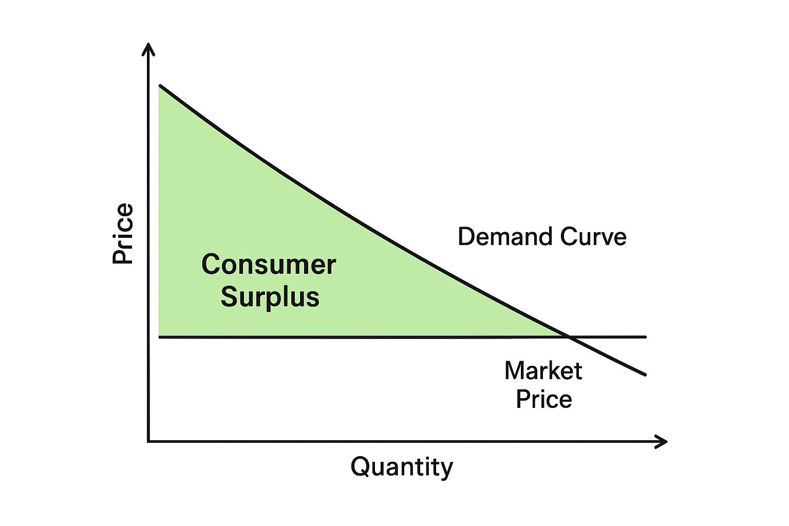
In this module, let us see an important application of limit: the Average Rate of Change, otherwise known as the Slope.

Recall:
PreAlgebra:
(1.) We defined slope as the ratio of the change in the output value of the function with respect to (wrt) a unit change in the input value of the function.
It is also known as the average rate of change.

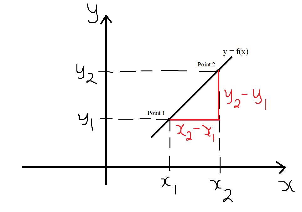
Considering a two-dimensional coordinate system where $y = f(x)$
y = dependent variable
x = independent variable

For a Linear Graph (Graph of a Linear Function) which is a straight line graph,

Graph of a Linear Function

$ \text{Point 1 } (x_1, y_1) \\[3ex] x_1 = \text{initial value of } x \\[3ex] y_1 = \text{initial value of } y \\[5ex] \text{Point 2 } (x_1, y_1) \\[3ex] x_2 = \text{final value of } x \\[3ex] y_2 = \text{final value of } y \\[3ex] \text{Change} = \text{final value} - \text{initial value} \\[3ex] \text{Change in } x = \Delta x = x_2 - x_1 \\[3ex] \text{Change in } y = \Delta y = y_2 - y_1 \\[3ex] \text{Slope, } m \\[3ex] = \dfrac{\Delta y}{\Delta x} \\[5ex] = \dfrac{y_2 - y_1}{x_2 - x_1} \\[5ex] $ In this example, both changes are positive.
Hence, the slope is also positive.
As the value of x increases, the value of y also increases.
This implies that the rate of change of y per unit change of x is positive.

Algebra:
(2.) We defined these terms:
(a.) The secant line to a curve is the line segment that intersects two points on the curve.
Secant Line

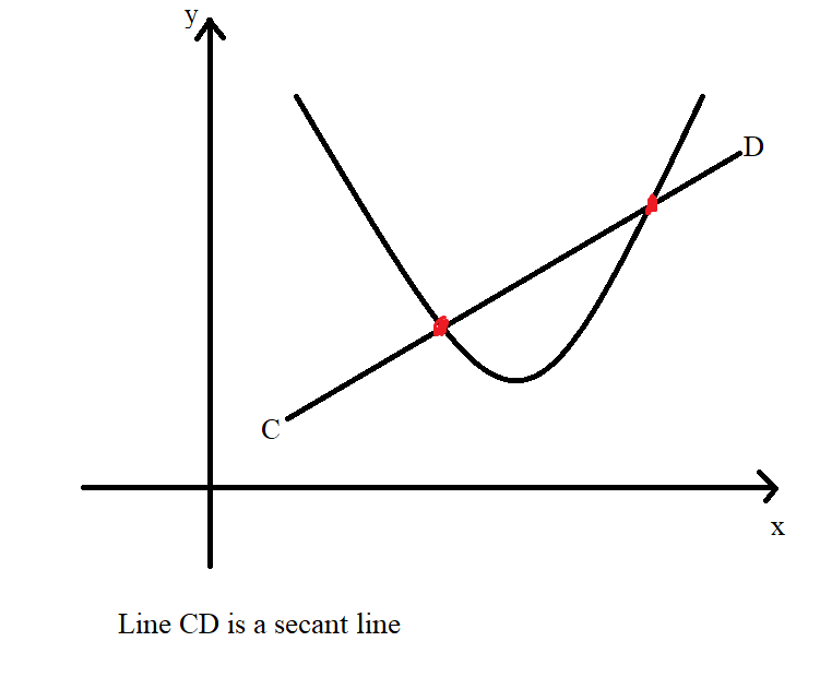
(b.) The tangent line to a curve is the line that touches only one point on the curve.
Tangent Line

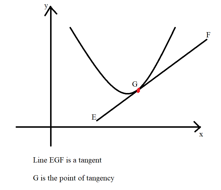
(Notice the terms: intersects, two points, touches, one point)

(3.) We reviewed the Difference Quotient of a function and noted these definitions.
We noted that:
(a.) The difference quotient of a function is the slope of the secant line.
(b.) The derivative of a function is the slope of the tangent line.

(4.) We also noted that for: the graph of all linear functions (straight-line graph): the slope of the line is the same at every point on the graph/line.
Depending on the graph, the slope can be positive, negative, zero, or undefined.

Calculus:
But, how do we find the slope of non-linear graphs (curves)?
For example, how do we find the slope of a: parabola? graph of a cubic function? graph of a quartic function? etc.
Well, here comes Calculus!
The derivative of the function, which is the slope of the tangent line is the limit of the difference quotient of the function.

Welcome to Average Rate of Change.

May you please:
(1.) Click the Week 2 module.
(2.) Review the Learning Objectives.
(3.) Review the Readings/Assessments.
(4.) Complete the assessments initially due this week.
(5.) Participate in the Week 2 Discussion (DB 2).
(6.) Attend the Live Sessions/Student Engagement Hours for this week.

Should you have any questions, please ask. I am here to help.
Thank you.

Samuel Chukwuemeka
Working together for success


Welcome to Week 3: Derivative by Limits and Derivative by Rules

Great Students,

Greetings to everyone.
Welcome to Module 3.

In Module 2, we discussed the average rate of change (slope).
We noted that the difference quotient of a function represents the slope of the secant line on its graph.
We also noted that the derivative of a function represents the slope of the tangent line on its graph.
In this module, we shall connect the Difference Quotient with the Derivative.
In other words, we will determine the derivative of a function based on its difference quotient.
Let us briefly revisit Module 1 on Limits.
The derivative of a function is the limit of its difference quotient as the independent variable approaches zero.
This is known as the Derivative by Limits, the Limit Definition of the Derivative, or the Derivative from First Principles.
In this module, we will find derivatives using the limit definition.
However, we do not always need to use limits to find derivatives.
We can also use a set of established rules, known as the Rules of Differentiation or Derivative by Rules.
In this module, we will focus on two of these Rules: the Power Rule and the Sum/Difference Rule.

Welcome to Derivative by Limits and Derivative by Rules.

May you please:
(1.) Click the Week 3 module.
(2.) Review the Learning Objectives.
(3.) Review the Readings/Assessments.
(4.) Complete the assessments initially due this week.
(5.) Review the course announcement: Applied Problems for DB 3
(6.) Participate in Week 3 Discussion (DB 3).
(7.) Attend the Live Sessions/Student Engagement Hours for this week.

Should you have any questions, please ask. I am here to help.
Thank you.

Samuel Chukwuemeka
Working together for success


Welcome to Week 4: Product Rule, Quotient Rule, and Chain Rule

Great Students,

Greetings to everyone.
Welcome to Module 4.

In Module 3, we discussed the Power Rule and the Sum/Difference Rule of Differentiation.
In this module, we will explore three additional Rules of Differentiation: the Product Rule, the Quotient Rule, and the Chain Rule.
As their names suggest:
The Product Rule is used when a function is expressed as the product of two or more terms.
The Quotient Rule is used when the function is expressed as a quotient of two terms.
What about the Chain Rule, also known as the Function of a Function Rule?
Why is it called the Chain Rule?
Why is it also referred to as the Function of a Function Rule?
When is it used?

Welcome to the Product Rule, Quotient Rule, and Chain Rule.

May you please:
(1.) Click the Week 4 module.
(2.) Review the Learning Objectives.
(3.) Review the Readings/Assessments.
(4.) Complete the assessments initially due this week.
(5.) Review the course announcement: Applied Problems for DB 4
(6.) Participate in Week 4 Discussion (DB 4).
(7.) Attend the Live Sessions/Student Engagement Hours for this week.

Should you have any questions, please ask. I am here to help.
Thank you.

Samuel Chukwuemeka
Working together for success


Welcome to Week 5: Higher-Order Derivatives, Natural Exponential Functions, and Natural Logarithmic Functions

Great Students,

Greetings to everyone.
Welcome to Module 5.

In Module 4, we discussed the Product Rule, the Quotient Rule, and the Chain Rule of Differentiation.
During the previous two weeks (Week 2 through Week 4), we determined the derivatives of functions using rules of differentiation.
Those derivatives are known as the first-order derivatives.
We can also have second-order, third-order, fourth-order, ... derivatives. These are known as higher-order derivatives.
In this module, we will find the higher-order derivatives of functions.
Next, we will discuss the natural exponential function: the exponential function with the Euler number base, e.
Further, we shall discuss the natural logarithmic function: the logarithmic function with the Euler number base, e.
So, what is e?
Say you deposit $1 in a financial institution that has an annual interest rate of 100% for 1 year.
Let us calculate the Amount for several options of times: annually, semiannually, quarterly, monthly, weekly, ordinary-daily, exact-daily, and several times per year.
We want to see how much you would get for each option of time for that same principal of $1 for that same time of 1 year.

Recall the Compound Amount Formula:

$ A = P\left(1 + \dfrac{r}{m}\right)^{mt} \\[5ex] P = \$1 \\[3ex] r = 100\% = \dfrac{100}{100} = 1 \\[5ex] t = 1\ \text{year} \\[3ex] $ In words:
If someone deposits an initial sum of money, $P$,
in a financial institution that pays an interest rate of $r\%$,
compounded $m$ times per year,
then after $t$ years,
the person will have an amount $A$.

Alternatively:
If someone borrows an initial sum of money, $P$,
from a financial institution that charges an interest rate of $r\%$,
compounded $m$ times per year,
then after $t$ years,
the person will owe an amount $A$.
Let us now calculate and observe.


Compounded: m A
Annually 1 $$ A = 1 * \left(1 + \dfrac{1}{1}\right)^{1 * 1} \\[5ex] A = 1(1 + 1)^1 \\[3ex] A = 1(2)^1 \\[3ex] A = 1(2) \\[3ex] A = \$2.00 $$
Semiannually 2 $$ A = 1 * \left(1 + \dfrac{1}{2}\right)^{2 * 1} \\[5ex] A = 1(1 + 0.5)^2 \\[3ex] A = 1(1.5)^2 \\[3ex] A = 1(2.25) \\[3ex] A = \$2.25 $$
Quarterly 4 $$ A = 1 * \left(1 + \dfrac{1}{4}\right)^{4 * 1} \\[5ex] A = 1(1 + 0.25)^4 \\[3ex] A = 1(1.25)^4 \\[3ex] A = 2.44140625 \\[3ex] A \approx \$2.44 $$
Monthly 12 $$ A = 1 * \left(1 + \dfrac{1}{12}\right)^{12 * 1} \\[5ex] A = 1(1 + 0.0833333333)^{12} \\[3ex] A = 1(1.0833333333)^{12} \\[3ex] A = 2.61303529 \\[3ex] A \approx \$2.61 $$
Weekly 52 $$ A = 1 * \left(1 + \dfrac{1}{52}\right)^{52 * 1} \\[5ex] A = 1(1 + 0.0192307692)^{52} \\[3ex] A = 1(1.019230769)^{52} \\[3ex] A = 2.692596954 \\[3ex] A \approx \$2.69 $$
Daily: Ordinary 360 $$ A = 1 * \left(1 + \dfrac{1}{360}\right)^{360 * 1} \\[5ex] A = 1(1 + 0.0027777778)^{360} \\[3ex] A = 1(1.002777778)^{360} \\[3ex] A = 2.714516025 \\[3ex] A \approx \$2.71 $$
Daily: Exact 365 $$ A = 1 * \left(1 + \dfrac{1}{365}\right)^{365 * 1} \\[5ex] A = 1(1 + 0.002739726)^{365} \\[3ex] A = 1(1.002739726)^{365} \\[3ex] A = 2.714567482 \\[3ex] A \approx \$2.71 $$
500 times per year 500 $$ A = 1 * \left(1 + \dfrac{1}{500}\right)^{500 * 1} \\[5ex] A = 1(1 + 0.002)^{500} \\[3ex] A = 1(1.002)^{500} \\[3ex] A = 2.715568521 \\[3ex] A \approx \$2.72 $$
1,000 times per year 1,000 $$ A = 1 * \left(1 + \dfrac{1}{1000}\right)^{1000 * 1} \\[5ex] A = 1(1 + 0.001)^{1000} \\[3ex] A = 1(1.001)^{1000} \\[3ex] A = 2.716923932 \\[3ex] A \approx \$2.72 $$
10,000 times per year 10,000 $$ A = 1 * \left(1 + \dfrac{1}{10000}\right)^{10000 * 1} \\[5ex] A = 1(1 + 0.0001)^{10000} \\[3ex] A = 1(1.0001)^{10000} \\[3ex] A = 2.718145927 \\[3ex] A \approx \$2.72 $$
100,000 times per year 100,000 $$ A = 1 * \left(1 + \dfrac{1}{100000}\right)^{100000 * 1} \\[5ex] A = 1(1 + 0.00001)^{100000} \\[3ex] A = 1(1.00001)^{100000} \\[3ex] A = 2.718268237 \\[3ex] A \approx \$2.72 $$
1,000,000 times per year 1,000,000 $$ A = 1 * \left(1 + \dfrac{1}{1000000}\right)^{1000000 * 1} \\[5ex] A = 1(1 + 0.000001)^{1000000} \\[3ex] A = 1(1.000001)^{1000000} \\[3ex] A = 2.718280469 \\[3ex] A \approx \$2.72 $$
10,000,000 times per year 10,000,000 $$ A = 1 * \left(1 + \dfrac{1}{10000000}\right)^{10000000 * 1} \\[5ex] A = 1(1 + 0.0000001)^{10000000} \\[3ex] A = 1(1.0000001)^{10000000} \\[3ex] A = 2.718281693 \\[3ex] A \approx \$2.72 $$

Observation:
From the table above, notice that when we compounded $1 (one dollar) 10,000 times per year, and then increased the compounding frequency up to 10,000,000 times per year, all within the same year, the first few digits of the resulting amount remained the same.
In each case, the amount was approximately $2.718$.
This constant value is known as the Euler number, named after the Swiss mathematician Leonhard Euler, and is also called Napier’s constant after the Scottish mathematician John Napier.
The number e is a fundamental mathematical constant that arises naturally in situations involving continuous growth or decay, and here it emerges from the limit of the compound interest formula as the compounding frequency approaches infinity.

Welcome to Higher-Order Derivatives, Natural Exponential Functions, and Natural Logarithmic Functions.

May you please:
(1.) Click the Week 5 module.
(2.) Review the Learning Objectives.
(3.) Review the Readings/Assessments.
(4.) Complete the assessments initially due this week.
(5.) Review the course announcement: Applied Problems for DB 5
(6.) Participate in Week 5 Discussion (DB 5).
(7.) Attend the Live Sessions/Student Engagement Hours for this week.

Should you have any questions, please ask. I am here to help.
Thank you.

Samuel Chukwuemeka
Working together for success


Welcome to Week 6: Derivatives of Natural Exponential Functions and Natural Logarithmic Functions

Great Students,

Greetings to everyone.
Welcome to Module 6.

In Module 5, we discussed the natural exponential functions and natural logarithmic functions.
We also derived the base of these functions: the Euler number constant.

In this module, we will determine the rate of change of these functions and then explore their applications in growth models: the uninhibited growth model and the inhibited growth model.

Uninhibited Growth Model: An example of this application is Continuous Compound Interest.
However, because as of today: 09/28/2025; there is no financial institution that compounds interest continuously (please let me know otherwise). The real-world example closest to continuous compounding is daily compounding.
Compound interest isn’t just a savings feature, it’s an engine for long-term growth. The more frequently your interest is compounded, the more often your balance earns money on top of money. Daily compounding gives your deposits a micro-boost every 24 hours, which can add up significantly over time.
(Source: Benzinga: Compound Interest Accounts for 2025: Daily Compounding, High APYs, and Smart Savings. )


Inhibited Growth Model (Logistic Function): An example of this application is Population Growth.
Let us review a case of yeast population growth in a nutrient-rich test tube.
When yeast cells are introduced into a fresh medium, their population initially grows rapidly (almost exponentially).
However, as nutrients are consumed and waste products accumulate, the growth rate slows.
Eventually, the population levels off at the carrying capacity, the maximum number of yeast cells the environment can sustain.
This is a case of logistic inhibited growth, where the growth curve is S-shaped:
Rapid growth at the start (plenty of resources).
Slowing growth as resources become limited.
Stabilization at the carrying capacity.
(Source: Biology LibreTexts, “Logistic Population Growth,” 2023 Biology LibreTexts )

Inhibited Growth Model (Piecewise Function): An example of this application is Salary Caps.
Samuel was hired as a 9-month Assistant Professor of Mathematics at Blue Ridge Community College in January, 2023.
Assume that he meets all the teaching faculty standards, maintains continuous employment, and earns an annual raise.
Using the 2024 – 2025 VCCS Salary Schedule
(a.) What is the maximum salary he can earn as an Assistant Professor of Mathematics?
(b.) If he is promoted to the higher rank, what is the maximum salary he can earn as an Associate Professor of Mathematics?
(c.) If he is promoted to the highest rank, what is the maximum salary he can earn as a Professor of Mathematics?

Welcome to the Derivatives of Natural Exponential Functions and Natural Logarithmic Functions.

May you please:
(1.) Click the Week 6 module.
(2.) Review the Learning Objectives.
(3.) Review the Readings/Assessments.
(4.) Complete the assessments initially due this week.
(5.) Review the course announcement: Applied Problems for DB 6
(6.) Participate in Week 6 Discussion (DB 6).
(7.) Attend the Live Sessions/Student Engagement Hours for this week.

Should you have any questions, please ask. I am here to help.
Thank you.

Samuel Chukwuemeka
Working together for success


Welcome to Week 7: Derivatives of Exponential Functions and Logarithmic Functions

Great Students,

Greetings to everyone.
Welcome to Module 7.

In Module 6, we discussed the applications of natural exponential functions in inhibited growth and uninhibited growth models.
In this module, we will explore another important application: exponential decay.

Exponential Decay Model in Archaeology: An example of this application is Radioactive Decay.
Radiocarbon dating, or carbon-14 dating, is a scientific method that can accurately determine the age of organic materials as old as approximately 60,000 years.
It is based on the fact that living organisms—like trees, plants, people, and animals—absorb carbon-14 into their tissue.
When they die, the carbon-14 starts to change into other atoms over time.
Scientists can estimate how long the organism has been dead by counting the remaining carbon-14 atoms.
Carbon-14 has a half-life of about 5,730 years.
That means half the atoms in a sample will change into other atoms, a process known as “decay,” in that amount of time.
(Source: University of Chicago News – "What is Carbon Dating"? )


Exponential Decay Model in Psychology: Another example of this application is Caffeine Elimination from the Human Body.
Raise your hand if you drink coffee daily. 😊
I drink coffee almost every day, though I don’t usually measure the amount.
After reading this, you might wonder whether it’s worth keeping track.

Scientists have found that between 250mg and 400mg per day of caffeine is the safest average dose range for most adults.
The body quickly absorbs and eliminates caffeine. Processed mainly through the liver, caffeine has a relatively short half-life: it takes about 5-7 hours, on average, to eliminate half of it from your body.
(Source: University of New Hampshire Psychological and Counseling Services (PACS) – "Caffeine: Uses, Abuses, Ups, and Downs". )


Additional research confirms this: (even though it is not from a tertiary institution)
In healthy people, the half-life of caffeine is about five hours, meaning it will take you around five hours, on average, to clear out 50% of the caffeine you consumed from your body.
(Source: People Inc. Health – "You Won’t Believe How Long Caffeine Can Affect You After Just One Cup". )

This implies that when a person consumes coffee or another caffeinated beverage, the caffeine concentration in the body decreases over time according to its half‑life.
For example:
After 5 hours, about 50% of the caffeine decays while 50% remains.
After 10 hours, about 25% decays while 25% remains.
After 15 hours, about 12.5% decays while 12.5% remains...and so on and so forth.
This exponential decay pattern helps doctors and researchers understand how long caffeine’s effects last and why late-day consumption can interfere with sleep.

Next, we will differentiate exponential functions and logarithmic functions.
Welcome to the Derivatives of Exponential Functions and Logarithmic Functions.

May you please:
(1.) Click the Week 7 module.
(2.) Review the Learning Objectives.
(3.) Review the Readings/Assessments.
(4.) Complete the assessments initially due this week.
(5.) Review the course announcement: Applied Problems for DB 7
(6.) Participate in Week 7 Discussion (DB 7).
(7.) Attend the Live Sessions/Student Engagement Hours for this week.

Should you have any questions, please ask. I am here to help.
Thank you.

Samuel Chukwuemeka
Working together for success


Welcome to Week 8: Relative Extrema and Derivative Tests

Great Students,

Greetings to everyone.
Welcome to Module 8.

In Module 7, we explored the applications of natural exponential functions in exponential decay models.
We also examined the derivatives of exponential and logarithmic functions.
In this module, we turn our attention to functions more broadly.
How do we make the best possible decisions using functions?
Consider two of the main goals of any business:
(1.) Maximize profits. (yes, even non-profit organizations).
Example: Sarah Technologies produces desktop computers.
The firm’s mathematician–economist determined that desktop sales during the summer season follow a polynomial model.
How many units should be sold during the summer to generate maximum revenue, and therefore maximum profit?


(2.) Minimize costs.
Example: Micah Farms typically orders citrus fertilizers during the winter season.
How many units of fertilizer should be ordered each month to minimize the total cost of producing citrus trees?


These are optimization problems, which lead us to the study of extrema (maximum and minimum values) of functions.
Extrema can be classified as:
Relative extrema (local maxima and local minima)
Absolute extrema (global maxima and global minima)
The First Derivative Test and the Second Derivative Test are tools for identifying relative extrema.
In this module, we will determine the relative extrema and sketch graphs of functions using these derivative tests.

Welcome to Relative Extrema and Derivative Tests.

May you please:
(1.) Click the Week 8 module.
(2.) Review the Learning Objectives.
(3.) Review the Readings/Assessments.
(4.) Complete the assessments initially due this week.
(5.) Review the course announcement: Applied Problems for DB 8.
(6.) Participate in Week 8 Discussion (DB 8).
(7.) Attend the Live Sessions/Student Engagement Hours for this week.

Should you have any questions, please ask. I am here to help.
Thank you.

Samuel Chukwuemeka
Working together for success


Welcome to Week 9: Optimization

Great Students,

Greetings to everyone.
Welcome to Module 9.

In Module 8, we determined the Relative Extrema of functions using the First Derivative Test and the Second Derivative Test.
In this module, we shall determine the Absolute Extrema of functions on closed intervals by applying the derivative tests and evaluating the function values at the endpoints of the interval.
This serves as a continuation of our study on using derivative tests (prior knowledge acquired in Module 8) and function values (prior knowledge acquired in Algebra) to solve optimization problems.
Think of this as moving from zooming in on local behavior (using derivative tests) to zooming out (combining derivative tests with endpoint evaluations) in order to see the big picture of a function’s maximum and minimum values.

Welcome to Optimization.

May you please:
(1.) Click the Week 9 module.
(2.) Review the Learning Objectives.
(3.) Review the Readings/Assessments.
(4.) Complete the assessments initially due this week.
(5.) Review the course announcement: Applied Problems for DB 9.
(6.) Participate in Week 9 Discussion (DB 9).
(7.) Attend the Live Sessions/Student Engagement Hours for this week.

Should you have any questions, please ask. I am here to help.
Thank you.

Samuel Chukwuemeka
Working together for success


Welcome to Week 10: Implicit Differentiation and Related Rates

Great Students,

Greetings to everyone.
Welcome to Module 10.

In the previous modules, we differentiated problems involving explicit functions: functions where the dependent variable, say y is expressed explicitly in terms of the independent variable, x.
For example: y = f(x)
In this module, we will differentiate implicit functions: functions where the dependent variable, say y is expressed implicitly in terms of the independent variable, x.
For example: f(x,y) = some expression involving x, y, xy, or a constant
This is known as Implicit Differentiation.

Next, we will discuss Related Rates.
Recall (Prior Knowledge): Function of a Function Rule
For variables say y, p, x:

$ \text{If } y = f(p) \\[3ex] \text{and } p = f(x) \\[3ex] \text{then, } \dfrac{dy}{dx} = \dfrac{dy}{dp} * \dfrac{dp}{dx}...\text{Chain Rule} \\[5ex] $ Now, let's connect it to Related Rates:

$ \dfrac{dy}{dt} = \dfrac{dy}{dx} * \dfrac{dx}{dt}...\text{Related Rates} \\[5ex] $ Here, we see that the rate of change of the dependent variable can be found from the rate of change of the independent variable and the derivative of the dependent variable with respect to the independent variable.

Welcome to Implicit Differentiation and Related Rates.

May you please:
(1.) Click the Week 10 module.
(2.) Review the Learning Objectives.
(3.) Review the Readings/Assessments.
(4.) Complete the assessments initially due this week.
(5.) Review the course announcement: Applied Problems for DB 10.
(6.) Participate in Week 10 Discussion (DB 10).
(7.) Attend the Live Sessions/Student Engagement Hours for this week.

Should you have any questions, please ask. I am here to help.
Thank you.

Samuel Chukwuemeka
Working together for success


Welcome to Week 11: Introduction to Integral Calculus

Great Students,

Greetings to everyone.
Welcome to Module 11.

So far, in modules 3 through 10, we have been working on Differential Calculus.
Recap: Given a function, we differentiated the function to get the derivative.
Now the natural question arises: Is it possible to reverse the process of differentiation in order to recover the original function?
The answer is yes.
This reverse process is called Integral Calculus. It is also known as Integration, the Antiderivative or Antidifferentiation.
Integration is also viewed as summation, so we use an elongated S to represent the integral, ∫

Student: Mr. C
I thought the sigma notation, Σ is used to represent summation.
Now, are you saying that the integral ∫ is also used to represent summation?
Do they mean the same thing? Can they be interchanged?
Teacher: Great question.
The sigma notation, Σ is a discrete sum.
It adds up separate, countable values.
Example: the sum of the mathematics test scores of students, one score at a time.
The integral, ∫ is a continuous sum.
It adds up infinitely many infinitesimal contributions across an interval.
Example: the total area under a curve that models student performance in mathematics across all possible scores.
So, both symbols represent summation, but in different contexts: Σ for discrete quantities, and ∫ for continuous quantities.
Another Analogy: Think of Σ as counting individual bricks, while ∫ is like pouring continuous cement.
They are related, but not interchangeable.


$ y = f(x)...\text{Function} \\[5ex] y' = f'(x) = \dfrac{dy}{dx} ...\text{Derivative of the Function} \\[7ex] \displaystyle\int f'(x)\;dx = f(x) ...\text{Integral of the Derivative gives back the Function} \\[7ex] \displaystyle\int f(x)\;dx ...\text{Integral of the Function} \\[5ex] $ We now have a basic idea of integration, so let us explore a situation where it can be applied.
Word Problem
A garden wall is built along a straight 2‑foot section of ground.
At the left end, the wall is 3 feet tall, and at the right end, it is 9 feet tall.
The top of the wall rises in a straight line between these two points, so the side profile of the wall forms a trapezoid.
Label the vertices with coordinates (0, 0) and (2, 0) for the bottom corners, and (0, 3) and (2, 9) for the top corners.
Algebra: Find the equation of the line representing the sloping top edge of the wall.
Coordinate Geometry: Sketch the graph and indicate the trapezoid formed by the ground (the base), the two vertical ends of the wall (the legs), and the sloping top edge.
Mensuration/Plane Geometry: Determine the area of this trapezoid using the trapezoid area formula.
Calculus: Calculate the area of the trapezoid using a definite integral, and compare your result with the geometric method.
Here is the solution to the problem.

Welcome to Introduction to Integral Calculus.

May you please:
(1.) Click the Week 11 module.
(2.) Review the Learning Objectives.
(3.) Review the Readings/Assessments.
(4.) Complete the assessments initially due this week.
(5.) Review the course announcement: Applied Problems for DB 11.
(6.) Participate in Week 11 Discussion (DB 11).
(7.) Attend the Live Sessions/Student Engagement Hours for this week.

Should you have any questions, please ask. I am here to help.
Thank you.

Samuel Chukwuemeka
Working together for success


Welcome to Week 12: Properties of Definite Integrals and Integration by Algebraic Substitution

Great Students,

Greetings to everyone.
Welcome to Module 12.

In the previous module, we solved an applied problem that involved the use of Power Rule to determine the antiderivative of a function.
We also evaluated its definite integral by applying the given lower and upper limits.

In this module, we will review the properties of definite integrals.
Then, we will apply another method of integration: algebraic substitution to integrate functions.

Welcome to Properties of Definite Integrals and Integration by Algebraic Substitution.

May you please:
(1.) Click the Week 12 module.
(2.) Review the Learning Objectives.
(3.) Review the Readings/Assessments.
(4.) Complete the assessments initially due this week.
(5.) Review the course announcement: Applied Problems for DB 12.
(6.) Participate in Week 12 Discussion (DB 12).
(7.) Attend the Live Sessions/Student Engagement Hours for this week.

Should you have any questions, please ask. I am here to help.
Thank you.

Samuel Chukwuemeka
Working together for success


Welcome to Week 13: Consumer and Producer Surpluses; Growth and Decay Models

Great Students,

Greetings to everyone.
Welcome to Module 13.

In the previous two modules, we integrated functions using the Power Rule and Algebraic Substitution.
We also evaluated definite integrals.
In this module, we will apply those integration techniques to integrate growth and decay models.
Additionally, we will use them to calculate consumer surplus and producer surplus.

Consumers demand goods and services, while producers supply them.
The interaction of demand and supply determines the market price.

In Economics, we often express the quantity of a product as a function of its price.
According to the Laws of Demand and Supply, ceteris paribus (everything else being constant):
(1) Demand: Quantity demanded is inversely related to price.
If price rises, the quantity demanded falls.
If price falls, the quantity demanded rises.

(2) Supply: Quantity supplied is directly related to price.
If price rises, the quantity supplied rises.
If price falls, the quantity supplied falls.

Thus, demand and supply are the two forces that determine the equilibrium price (the price at which the quantity demanded is equal to the quantity supplied) and the quantity of a product.

In Calculus, price can be expressed as a function of quantity, which allows us to calculate surplus areas.
(1) Demand Curve: This shows the inverse relationship between price and quantity demanded.
Consumer Surplus: The difference between what consumers are willing to pay and what they actually pay.
Graphically, it is the area between the demand curve and the market price line.

Consumer Surplus
(Image is generated using: https://copilot.microsoft.com/)

(2) Supply Curve: This shows the direct relationship between price and quantity supplied.
Producer Surplus: The difference between the price producers receive and the minimum price they would accept.
Graphically, it is the area between the supply curve and the market price line.

Producer Surplus
(Image is generated using: https://copilot.microsoft.com/)

Is it feasible to have a point where the demand and supply curves intersect?
Welcome to Consumer and Producer Surplus; Growth and Decay Models.

May you please:
(1.) Click the Week 13 module.
(2.) Review the Learning Objectives.
(3.) Review the Readings/Assessments.
(4.) Complete the assessments initially due this week.
(5.) Review the course announcement: Applied Problems for DB 13.
(6.) Participate in Week 13 Discussion (DB 13).
(7.) Attend the Live Sessions/Student Engagement Hours for this week.

Should you have any questions, please ask. I am here to help.
Thank you.

Samuel Chukwuemeka
Working together for success